Three basic concepts are key to producing all types of fractals: iteration, formulas, and orbits. In this essay, we’ll explore what these mean and how they work to produce fractals. But first we make an observation and define two important terms.
The observation: Fractals are infinite. Computers are finite. So any image we create using a fractal program can only be an approximation of the underlying fractal.
This leads to the first term: Render. To render a fractal simply means to create an image of the fractal. This simple definition belies the complexity of the process and the artistic decisions associated with rendering, but elaborating on those details will need to wait for another post. For our purposes here, rendering is the magic that takes all of the options we’ve selected in our fractal program (the formulas, colors, location, etc.) and turns them into a picture.
The second important term: Parameters; params for short. These are the options we’ve selected in our fractal program in a textual form that we can save in a file or copy/paste to a social media site to share with others. They aren’t much to look at, but they describe the infinite fractal and can be reloaded and re-rendered. More importantly, they can be used as a starting point to make new fractals by loading them and changing the options.
Iteration simply means repeating something over and over, and is the way all fractals are defined. For example, consider the procedure described by Swedish mathematician Niels Fabian Helge von Koch in 1904 for creating a fractal known as the “Koch snowflake”:
Step 0. Start with an equilateral triangle.
Step 1. Do the following for each of the three lines in the triangle:
a. Divide the line into three equal segments.
b. Replace the middle segment with an equilateral triangle that points outward and has that segment as its base.
c. Remove the middle segment.
Step 2. Repeat steps a-c for each of the 12 smaller lines of the resulting figure.
Step 3. Repeat steps a-c for each of the 48 lines of the resulting figure.
…
Step n. Repeat steps a-c for each of the 3×4^(n−1) lines of the resulting figure.
…
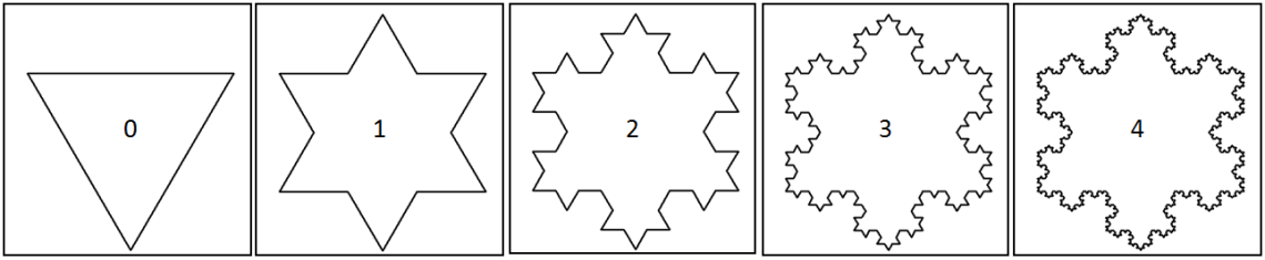
The figure shows the results of steps 0 through 4. As this scale, we can barely see the added details of step 4, and they are completely lost at higher steps. So we can stop our finite approximation there. But the fractal itself is infinite. Details of later steps would be visible if we were to zoom in to a part of the fractal and iterate enough times. In fact, the boundary of the infinite snowflake would look exactly the same no matter how far we zoom in, taking rotation and shifting into account. This self similarity is a hallmark of fractals.Another interesting property of this and many other fractals is that the boundary is infinitely long, but it encloses a finite area.
Although iterating geometric constructions is an interesting way to make fractals, most fractal art programs work by iterating formulas, also known as functions, transforms, and mappings. In general, we’ll use these terms interchangably. The formulas used to make fractals always map a point to another point. Iteration is done by repeating the formula, mapping the second point to a third point, and the third point to a fourth point, and so on.
To understand this concept, let’s start with one dimensional points, which are just numbers, and use a calculator with the function key 
| Starting Value | Orbit |
| 0 | 0, 0, 0, 0, … |
| 0.5 | 0.25, 0.0625, 0.00390625, 0.0000152587890625, … |
| 0.75 | 0.5625, 0.31640625, 0.1001129150390625, … |
| 1 | 1, 1, 1, 1, … |
| 1.5 | 2.25, 5.0625, 25.62890625, 656.8408355712890625, … |
| 2 | 4, 16, 256, 65536, … |
| 10 | 100, 10000, 100000000, 10000000000000000,… |
Orbits are always infinite, and are generally different for each starting value. The orbits here have some interesting properties.
- The orbits for 0 and 1 repeat that value indefinitely.
- Orbits for values between 0 and 1 get closer and closer to 0 (but never quite reach it).
- Orbits for values greater than 1 get very large very quickly; they approach ∞.
- Orbits for values less than 0 aren’t shown in the table, but they are the same as their positive counterparts. For example, the orbit for -1 is 1, 1, 1, …, just like 1.
To make fractals, we need more interesting formulas. We also use points in two or three dimensions since one dimensional fractals are rather boring visually. It is these fractal formulas that we will explore in the Fractal Formulas blog.
There are a number of formats used to express formulas; we’ll use
This is pronounced “f of x equals x squared”. Different letters can be used, especially when discussing multiple functions. For example, 
The next notation makes the iteration more clear by using a subscript to indicate the orbit sequence: 


This is pronounced “x sub n equals x sub n minus 1 squared”. It expresses the next orbit point in terms of the previous one. It is especially useful for the occasional formulas that depend on several previous orbit points (for example, 


Another notation occasionally seen is the following:

This is pronounced “x maps to x squared”, and emphasizes the mapping aspect of the formula.
We will mention one final formula notation since it can be confusing:

This is a computer programming notation; the ‘=’ is the assignment operator, so this would be pronounced “x is assigned x squared”. Taken out of context, it can be mistaken for an algebraic equation where you need to find the value of x that makes the equation true. It would actually more likely be written as “x = x ^ 2” since programming languages don’t have italics or superscripts, and the surrounding code would make it clear that this is part of a program.
So orbits come from iterating formulas. Let’s see how they can be used to create fractals. One way is to use the orbit as the fractal itself; these are called orbital fractals. This isn’t really meaningful if every starting point has a completely different orbit (like 

A more popular type of orbital fractal is the flame fractal, which uses several functions (usually called tranformations or transforms in flame fractal software). For each iteration, one of the functions is chosen randomly, so the precise orbit is unpredictable, but when iterated many thousands of times the randomness averages out and a consistent fractal is generated. The following flame fractal uses three transforms to generate a fractal snowflake.

Another common way to use orbits to create fractals is to separate points into two sets, depending on whether their orbits stay within some boundary or go off to infinity. For example, with our earlier example f(x)=x^2, points between -1 and 1 have bounded orbits and other points have orbits whose values get larger and larger without limit. We call the points with bounded orbits inside points because they belong to the “filled-in Julia set” of the formula, after French mathematician Gaston Julia. (The filled-in Julia set is often just called the Julia set for convenience, though technically the Julia set is the boundary of the filled-in Julia set.) Conversely, the points whose orbits are not bounded are called outside points.
When rendering this kind of fractal, we need to set some boundaries to keep the orbits finite. We need two of them:
- An escape condition for the orbit, such as a maximum distance from the origin. This is also called a bailout condition. If the escape condition is reached while computing the orbit of a point, we assume the orbit is unbounded so the point is outside.
- A maximum orbit length or maximum iterations. If the escape condition is not reached before the orbit reaches its maximum length, we assume the orbit is bounded so the point is inside.
Color is not part of the mathematical definition of a fractal, but we often want to add some color (or at least shades of gray) to make the pictures more interesting. One way to do this is to base the color on the length of the orbit before the escape condition is reached, called the “escape time”, giving these fractals the name escape time fractal. This method is useful because outside points that are close to the fractal take longer to escape than points that are further away.
In the following fractal, the inside is black and the outside is colored by the escape time, with points closer to the inside darker and points further away lighter.
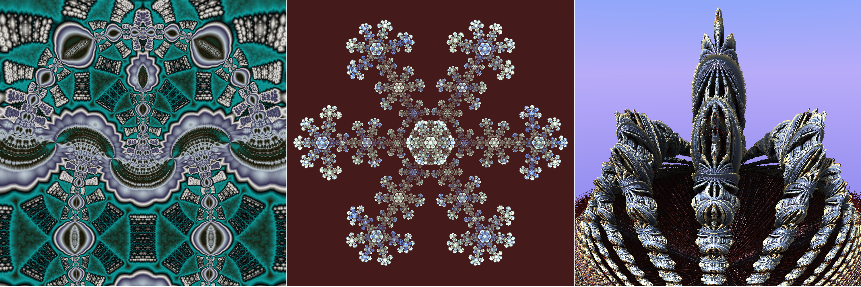
Here is another escape time fractal known as a “Ducky” (I don’t know where that name came from). The formula is very different from the last one; it has an inherent symmetry that is repeated at different levels and orientations as it is iterated, producing complex but symmetrical patterns. This one doesn’t have inside and outside points (all the points are “inside”), and coloring is based on statistics of the orbit points.

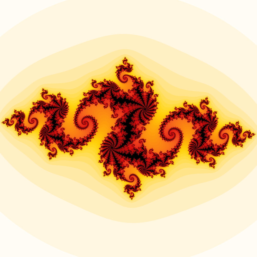
Three dimensional fractals work much the same as two dimensional ones: we iterate a formula using three dimensional points. The result is projected to two dimensions for display or printing by pointing a virtual camera at the fractal. For three dimensional orbital fractals, that’s all there is to it. Here is a simple three dimensional flame fractal that resembles a flower; you can see how the iterated function makes the petals smaller and smaller:

Escape time fractals are quite different in three dimensions. Outside points need to remain transparent; we wouldn’t be able to see anything if they were colored according to their escape time (consider what the world would be like if air was opaque). What we really want to see is the surface of the fractal, where inside meets outside. The usual method for rendering these fractals is called ray marching. Without going into a lot of detail, ray marching shoots a ray from each camera pixel toward the fractal to see how far away it is. Since points closer to the fractal have a higher escape time, the distance to the fractal can be estimated, which is used to march the ray closer until it reaches the fractal surface and the point can be colored. Lighting techniques from 3D modeling tools are used to give the fractal a 3D appearance.
Here is a fractal made using this method:

There are other methods for making fractals, but these are the ones most commonly used by fractal artists. Hopefully this provides some background that will be helpful as we explore Fractal Formulas.
